9.5 Real Distribution Families
The distribution object constructors documented in this section return uniquely defined distributions for the largest possible parameter domain. This usually means that they return distributions for a larger domain than their mathematical counterparts are defined on.
> (pdf (normal-dist 1 0) 1) +inf.0
> (pdf (normal-dist 1 0) 1.0000001) 0.0
Some parameters’ boundary values give rise to non-unique limits. Sometimes the ambiguity can be resolved using necessary properties; see Gamma-Dist for an example. When no resolution exists, as with (beta-dist 0 0), which puts an indeterminate probability on the value 0 and the rest on 1, the constructor returns an undefined distribution.
Some distribution object constructors attempt to return sensible distributions when given special values such as +inf.0 as parameters. Do not count on these yet.
Many distribution families, such as Gamma-Dist, can be parameterized on either scale or rate (which is the reciprocal of scale). In all such cases, the implementations provided by math/distributions are parameterized on scale.
9.5.1 Beta Distributions
Wikipedia: Beta Distribution.
syntax
procedure
alpha : Real beta : Real
procedure
(beta-dist-alpha d) → Flonum
d : Beta-Dist
procedure
(beta-dist-beta d) → Flonum
d : Beta-Dist
Examples: | ||||||||||||||||
|
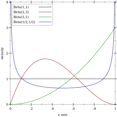
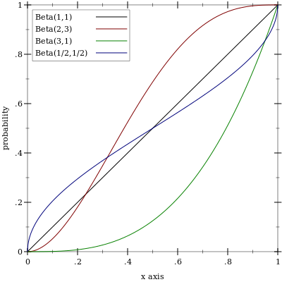
(beta-dist 0 0) and (beta-dist +inf.0 +inf.0) are undefined distributions.
When a = 0 or b = +inf.0, the returned distribution acts like (delta-dist 0).
When a = +inf.0 or b = 0, the returned distribution acts like (delta-dist 1).
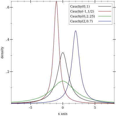
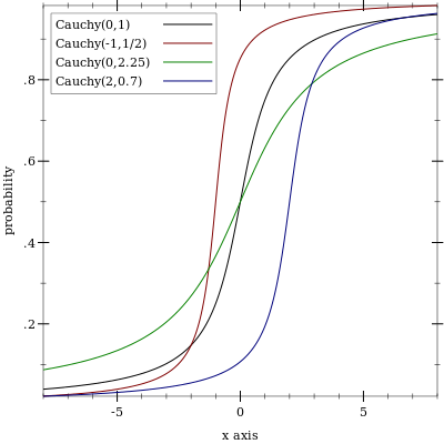
9.5.2 Cauchy Distributions
Wikipedia: Cauchy Distribution.
syntax
procedure
(cauchy-dist [mode scale]) → Cauchy-Dist
mode : Real = 0 scale : Real = 1
procedure
(cauchy-dist-mode d) → Flonum
d : Cauchy-Dist
procedure
(cauchy-dist-scale d) → Flonum
d : Cauchy-Dist
Examples: | |||||||||||||||||
|
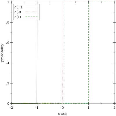
9.5.3 Delta Distributions
Wikipedia: Dirac Delta Function.
syntax
procedure
(delta-dist [mean]) → Delta-Dist
mean : Real = 0
procedure
(delta-dist-mean d) → Flonum
d : Delta-Dist
Examples: | |||||||||||
|
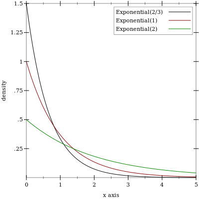
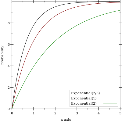
9.5.4 Exponential Distributions
Wikipedia: Exponential Distribution.
syntax
procedure
(exponential-dist [mean]) → Exponential-Dist
mean : Real = 1
procedure
(exponential-dist-mean d) → Flonum
d : Exponential-Dist
(exponential-dist (/ 1.0 rate))
Examples: | ||||||||||||||||
|
9.5.5 Gamma Distributions
Wikipedia: Gamma Distribution.
syntax
procedure
(gamma-dist [shape scale]) → Gamma-Dist
shape : Real = 1 scale : Real = 1
procedure
(gamma-dist-shape d) → Flonum
d : Gamma-Dist
procedure
(gamma-dist-scale d) → Flonum
d : Gamma-Dist
(gamma-dist shape (/ 1.0 rate))
Examples: | ||||||||||||||||||
|
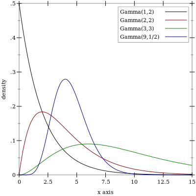
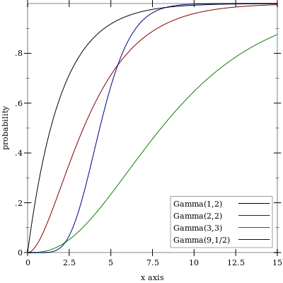
> (cdf (gamma-dist 0 1) 0) 1.0
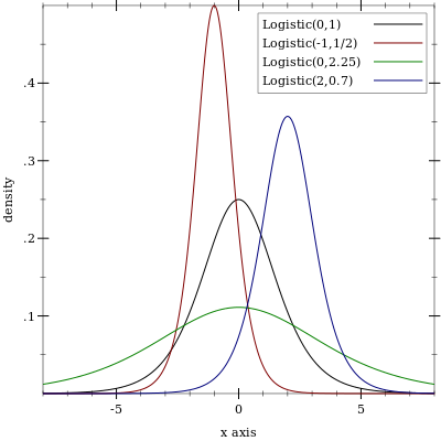
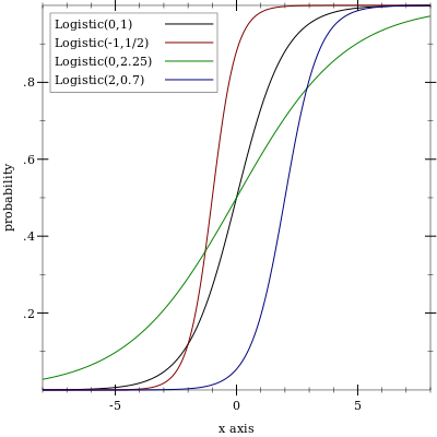
9.5.6 Logistic Distributions
Wikipedia: Logistic Distribution.
syntax
procedure
(logistic-dist [mean scale]) → Logistic-Dist
mean : Real = 0 scale : Real = 1
procedure
(logistic-dist-mean d) → Flonum
d : Logistic-Dist
procedure
(logistic-dist-scale d) → Flonum
d : Logistic-Dist
Examples: | |||||||||||||||||
|
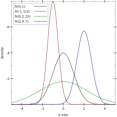
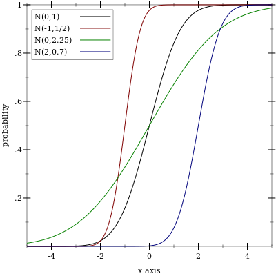
9.5.7 Normal Distributions
Wikipedia: Normal Distribution.
syntax
procedure
(normal-dist [mean stddev]) → Normal-Dist
mean : Real = 0 stddev : Real = 1
procedure
(normal-dist-mean d) → Flonum
d : Normal-Dist
procedure
(normal-dist-stddev d) → Flonum
d : Normal-Dist
(normal-dist mean (sqrt var))
Examples: | ||||||||||||||||
|
9.5.8 Triangular Distributions
Wikipedia: Triangular Distribution.
syntax
procedure
(triangle-dist [min max mode]) → Triangle-Dist
min : Real = 0 max : Real = 1 mode : Real = (* 0.5 (+ min max))
procedure
(triangle-dist-min d) → Flonum
d : Triangle-Dist
procedure
(triangle-dist-max d) → Flonum
d : Triangle-Dist
procedure
(triangle-dist-mode d) → Flonum
d : Triangle-Dist
If min, mode and max are not in ascending order, they are sorted before constructing the distribution object.
Examples: | ||||||||||||||||||
|
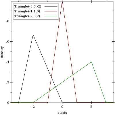
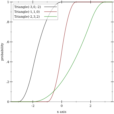
(triangle-dist c c c) for any real c behaves like a support-limited delta distribution centered at c.
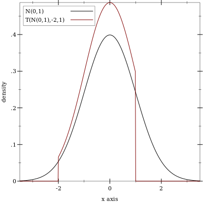
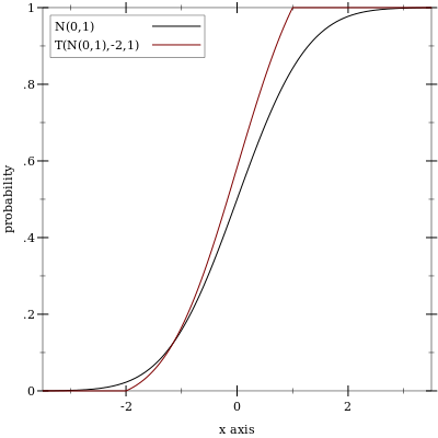
9.5.9 Truncated Distributions
syntax
procedure
(truncated-dist d) → Truncated-Dist
d : Real-Dist (truncated-dist d max) → Truncated-Dist d : Real-Dist max : Real (truncated-dist d min max) → Truncated-Dist d : Real-Dist min : Real max : Real
procedure
t : Truncated-Dist
procedure
(truncated-dist-min t) → Flonum
t : Truncated-Dist
procedure
(truncated-dist-max t) → Flonum
t : Truncated-Dist
(truncated-dist d) is equivalent to (truncated-dist d -inf.0 +inf.0). (truncated-dist d max) is equivalent to (truncated-dist d -inf.0 max). If min > max, they are swapped before constructing the distribution object.
Samples are taken by applying the truncated distribution’s inverse cdf to uniform samples.
Examples: | ||||||||||||||||||
|
9.5.10 Uniform Distributions
Wikipedia: Uniform Distribution.
syntax
procedure
(uniform-dist max) → Uniform-Dist max : Real (uniform-dist min max) → Uniform-Dist min : Real max : Real
procedure
(uniform-dist-min d) → Flonum
d : Uniform-Dist
procedure
(uniform-dist-max d) → Flonum
d : Uniform-Dist
(uniform-dist) is equivalent to (uniform-dist 0 1). (uniform-dist max) is equivalent to (uniform-dist 0 max). If max < min, they are swapped before constructing the distribution object.
Examples: | ||||||||||||||||
|
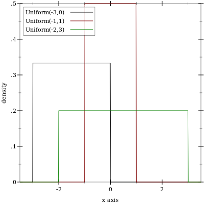
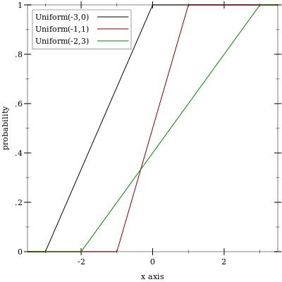
(uniform-dist x x) for any real x behaves like a support-limited delta distribution centered at x.