9 Tree Layout

These functions specify tree layouts and functions that render them as picts.

package: pict-lib

procedure
(tree-layout [#:pict node-pict] child ...) → tree-layout?
node-pict : (or/c #f pict?) = #f
child : (or/c tree-layout? tree-edge? #f)

Specifies an interior node of a tree for use with one of the renderers below.

If the children are tree-layout?s, then they have edges created by passing the corresponding tree-layout?s directly to tree-edge. Children that are #f correspond to leaf nodes that are not drawn.

The default node-pict (used when it is #f) is

procedure
(tree-edge node [#:edge-color edge-color]) → tree-edge?
  node : tree-layout?
   edge-color :
(or/c string?
      (is-a?/c color%)
      (list/c byte? byte? byte?))
= "gray"

This function specifies an edge from some parent to the given node. It it intended to be used with tree-layout.

procedure
(tree-layout? v) → boolean?
v : any/c

Recognizes a tree layout. It returns #t when given #f or the result of tree-layout.

procedure
(binary-tree-layout? v) → boolean?
v : any/c

Recognizes a tree-layout? that represents a binary tree. That is, each interior node has either two children or is #f. Note that a node with zero children does not count as a leaf for the purposes of binary-tree-layout?.

Examples:

> (binary-tree-layout? (tree-layout #f #f))
#t
> (binary-tree-layout? #f)
#t
> (binary-tree-layout? (tree-layout (tree-layout) (tree-layout)))
#f

procedure
(tree-edge? v) → boolean?
v : any/c

Recognizes an tree-edge.

procedure
(naive-layered tree-layout
[ #:x-spacing x-spacing
#:y-spacing y-spacing]) → pict?
  tree-layout : tree-layout?
  x-spacing : (or/c (and/c real? positive?) #f) = #f
  y-spacing : (or/c (and/c real? positive?) #f) = #f

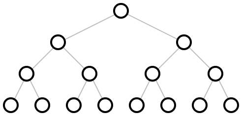
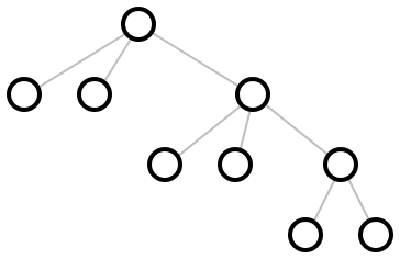
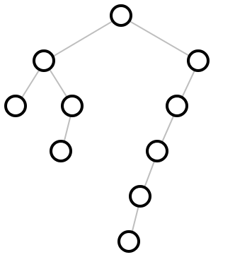
Uses a naive algorithm that ensures that all nodes at a fixed depth are the same vertical distance from the root (dubbed “layered”). It recursively lays out subtrees and then horizontally combines them, aligning them at their tops. Then it places the root node centered over the children nodes.

Examples:

> (define (complete d)
    (cond
      [(zero? d) #f]
      [else (define s (complete (- d 1)))
            (tree-layout s s)]))
> (naive-layered (complete 4))
> (naive-layered (tree-layout
                  (tree-layout)
                  (tree-layout)
                  (tree-layout
                   (tree-layout)
                   (tree-layout)
                   (tree-layout
                    (tree-layout)
                    (tree-layout)))))
> (define right-subtree-with-left-chain
    (tree-layout
     (tree-layout
      (tree-layout #f #f)
      (tree-layout
       (tree-layout #f #f)
       #f))
     (tree-layout
      (tree-layout
       (tree-layout
        (tree-layout
         (tree-layout #f #f)
         #f)
        #f)
       #f)
      #f)))
> (naive-layered right-subtree-with-left-chain)

procedure
(binary-tidier tree-layout
[ #:x-spacing x-spacing
#:y-spacing y-spacing]) → pict?
  tree-layout : binary-tree-layout?
  x-spacing : (or/c (and/c real? positive?) #f) = #f
  y-spacing : (or/c (and/c real? positive?) #f) = #f

Uses the layout algorithm from Tidier Drawing of Trees by Edward M. Reingold and John S. Tilford (IEEE Transactions on Software Engineering, Volume 7, Number 2, March 1981) to lay out tree-layout.

The layout algorithm guarantees a number of properties, namely:

nodes at the same level of tree appear at the same vertical distance from the top of the pict
parents are centered over their children, which are placed from left to right,
isomorphic subtrees are drawn the same way, no matter where they appear in the complete tree, and
a tree and its mirror image produce picts that are mirror images of each other (which also holds for subtrees of the complete tree).

Within those constraints, the algorithm tries to make as narrow a drawing as it can, even to the point that one subtree of a given node might cross under the other one.

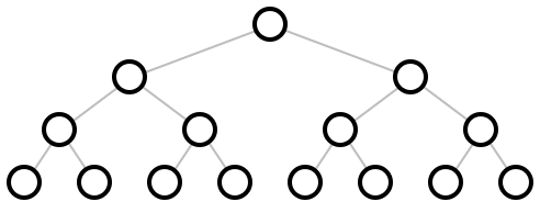
More precisely, it recursively lays out the two subtree and then, without adjusting the layout of the two subtrees, moves them as close together as it can, putting the root of the new tree centered on top of its children. (It does this in linear time, using clever techniques as discussed in the paper.)

The x-spacing and y-spacing are the amount of space that each row and each column takes up, measured in pixels. If x-spacing is #f, it is the width of the widest node pict? in the tree. If y-spacing is #f, it is 1.5 times the width of the widest node pict? in the tree.

Examples:

> (binary-tidier (complete 4))
> (define (dl t) (tree-layout (tree-layout #f #f) t))
> (define (dr t) (tree-layout t (tree-layout #f #f)))
> (binary-tidier
   (tree-layout
    (dr (dr (dr (dl (dl (dl (complete 2)))))))
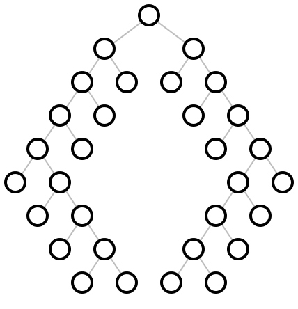
    (dl (dl (dl (dr (dr (dr (complete 2)))))))))
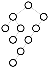
> (binary-tidier right-subtree-with-left-chain)

procedure
(hv-alternating tree-layout
[ #:x-spacing x-spacing
#:y-spacing y-spacing]) → pict?
  tree-layout : binary-tree-layout?
  x-spacing : (or/c (and/c real? positive?) #f) = #f
  y-spacing : (or/c (and/c real? positive?) #f) = #f

Uses the “CT” binary tree layout algorithm from A note on optimal area algorithms for upward drawing of binary trees by P. Crescenzi, G. Di Battista, and A. Piperno (Computational Geometry, Theory and Applications, 1992) to lay out tree-layout.

It adds horizontal and vertical space between layers based on x-spacing and y-spacing. If either is #f, 1.5 times the size of the biggest node is used.

Example:

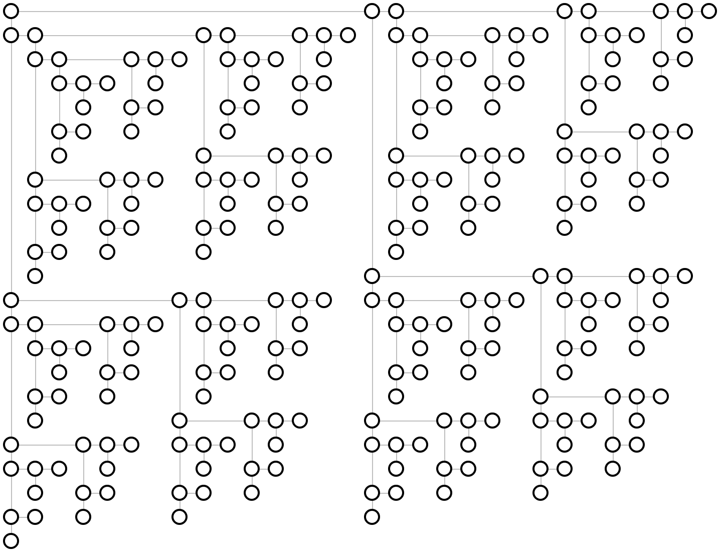
> (hv-alternating (complete 8))

Added in version 6.0.1.4 of package pict-lib.

top ← prev up next →

1	Pict Datatype
2	Basic Pict Constructors
3	Pict Combiners
4	Pict Drawing Adjusters
5	Bounding Box Adjusters
6	Pict Finders
7	More Pict Constructors
8	Animation Helpers
9	Tree Layout
10	Miscellaneous
11	Rendering
12	Conversion to Picts